Receiving BPSK symbols (Part 3/5) 🐀

In the last post, we worked through how to generate a BPSK signal, and hopefully transmit it using one of our SDRs. Let’s take that and move on to Receiving BPSK and turning that back into symbols!

Demodulating BPSK data is a bit more tricky than transmitting BPSK data, mostly due to tedious facts of life such as space, time, and hardware built with compromises because not doing that makes the problem impossible. Unfortunately, it’s now our job to work within our imperfect world to recover perfect data. We need to handle the addition of noise, differences in frequency, clock synchronization and interference in order to recover our information. This makes life a lot harder than when we transmit information, and as a result, a lot more complex.

Coarse Sync

Our starting point for this section will be working from a capture of a number of generated PACKRAT packets as heard by a PlutoSDR at (xz compressed interleaved int16, 2,621,440 samples per second)

Every SDR has its own oscillator, which eventually controls a number of different components of an SDR, such as the IF (if it’s a superheterodyne architecture) and the sampling rate. Drift in oscillators lead to drifts in frequency – such that what one SDR may think is 100MHz may be 100.01MHz for another radio. Even if the radios were perfectly in sync, other artifacts such as doppler time dilation due to motion can cause the frequency to appear higher or lower in frequency than it was transmitted.

All this is a long way of saying, we need to determine when we see a strong signal that’s close-ish to our tuned frequency, and take steps to roughly correct it to our center frequency (in the order of 100s of Hz to kHz) in order to acquire a phase lock on the signal to attempt to decode information contained within.

The easiest way of detecting the loudest signal of interest is to use an FFT. Getting into how FFTs work is out of scope of this post, so if this is the first time you’re seeing mention of an FFT, it may be a good place to take a quick break to learn a bit about the time domain (which is what the IQ data we’ve been working with so far is), frequency domain, and how the FFT and iFFT operations can convert between them.

Lastly, because FFTs average power over the window, swapping phases such that the transmitted wave has the same number of in-phase and inverted-phase symbols the power would wind up averaging to zero. This is not helpful, so I took a tip from Dr. Marc Lichtman’s PySDR project and used complex squaring to drive our BPSK signal into a single detectable carrier by squaring the IQ data. Because points are on the unit circle and at tau/2 (specifically, tau/(2^1) for BPSK, 2^2 for QPSK) angles, and given that squaring has the effect of doubling the angle, and angles are all mod tau, this will drive our wave comprised of two opposite phases back into a continuous wave – effectively removing our BPSK modulation, making it much easier to detect in the frequency domain. Thanks to Tom Bereknyei for helping me with that!

...
  var iq []complex{}
  var freq []complex{}

  for i := range iq {
      iq[i] = iq[i] * iq[i]
  }

  // perform an fft, computing the frequency
  // domain vector in `freq` given the iq data
  // contained in `iq`.
  fft(iq, freq)

  // get the array index of the max value in the
  // freq array given the magnitude value of the
  // complex numbers.
  var binIdx = max(abs(freq))
...

Now, most FFT operations will lay the frequency domain data out a bit differently than you may expect (as a human), which is that the 0th element of the FFT is 0Hz, not the most negative number (like in a waterfall). Generally speaking, “zero first” is the most common frequency domain layout (and generally speaking the most safe assumption if there’s no other documentation on fft layout). “Negative first” is usually used when the FFT is being rendered for human consumption – such as a waterfall plot.

Given that we now know which FFT bin (which is to say, which index into the FFT array) contains the strongest signal, we’ll go ahead and figure out what frequency that bin relates to.

In the time domain, each complex number is the next time instant. In the frequency domain, each bin is a discrete frequency – or more specifically – a frequency range. The bandwidth of the bin is a function of the sampling rate and number of time domain samples used to do the FFT operation. As you increase the amount of time used to perform the FFT, the more precise the FFT measurement of frequency can be, but it will cover the same bandwidth, as defined by the sampling rate.

...
  var sampleRate = 2,621,440

  // bandwidth is the range of frequencies
  // contained inside a single FFT bin,
  // measured in Hz.
  var bandwidth = sampleRate/len(freq)
...

Now that we know we have a zero-first layout and the bin bandwidth, we can compute what our frequency offset is in Hz.

...
  // binIdx is the index into the freq slice
  // containing the frequency domain data.
  var binIdx = 0

  // binFreq is the frequency of the bin
  // denoted by binIdx
  var binFreq = 0

  if binIdx > len(freq)/2 {
    // This branch covers the case where the bin
    // is past the middle point - which is to say,
    // if this is a negative frequency.
    binFreq = bandwidth * (binIdx - len(freq))
  } else {
    // This branch covers the case where the bin
    // is in the first half of the frequency array,
    // which is to say - if this frequency is
    // a positive frequency.
    binFreq = bandwidth * binIdx
  }
...

However, sice we squared the IQ data, we’re off in frequency by twice the actual frequency – if we are reading 12kHz, the bin is actually 6kHz. We need to adjust for that before continuing with processing.

...
  var binFreq = 0

  ...
  // [compute the binFreq as above]
  ...

  // Adjust for the squaring of our IQ data
  binFreq = binFreq / 2
...

Finally, we need to shift the frequency by the inverse of the binFreq by generating a carrier wave at a specific frequency and rotating every sample by our carrier wave – so that a wave at the same frequency will slow down (or stand still!) as it approaches 0Hz relative to the carrier wave.

  var tau = pi * 2

  // ts tracks where in time we are (basically: phase)
  var ts float

  // inc is the amount we step forward in time (seconds)
  // each sample.
  var inc float = (1 / sampleRate)

  // amount to shift frequencies, in Hz,
  // in this case, shift +12 kHz to 0Hz
  var shift = -12,000

  for i := range iq {
    ts += inc
    if ts > tau {
      // not actually needed, but keeps ts within
      // 0 to 2*pi (since it is modulus 2*pi anyway)
      ts -= tau
    }

    // Here, we're going to create a carrier wave
    // at the provided frequency (in this case,
    // -12kHz)
    cwIq = complex(cos(tau*shift*ts), sin(tau*shift*ts))

    iq[i] = iq[i] * cwIq
  }

Now we’ve got the strong signal we’ve observed (which may or may not be our BPSK modulated signal!) close enough to 0Hz that we ought to be able to Phase Lock the signal in order to begin demodulating the signal.

Filter

After we’re roughly in the neighborhood of a few kHz, we can now take some steps to cut out any high frequency components (both positive high frequencies and negative high frequencies). The normal way to do this would be to do an FFT, apply the filter in the frequency domain, and then do an iFFT to turn it back into time series data. This will work in loads of cases, but I’ve found it to be incredibly tricky to get right when doing PSK. As such, I’ve opted to do this the old fashioned way in the time domain.

I’ve – again – opted to go simple rather than correct, and haven’t used nearly any of the advanced level trickery I’ve come across for fear of using it wrong. As a result, our process here is going to be generating a sinc filter by computing a number of taps, and applying that in the time domain directly on the IQ stream.

// Generate sinc taps

func sinc(x float) float {
  if x == 0 {
    return 1
  }
  var v = pi * x
  return sin(v) / v
}

...
  var dst []float
  var length = float(len(dst))

  if int(length)%2 == 0 {
    length++
  }

  for j := range dst {
    i := float(j)
    dst[j] = sinc(2 * cutoff * (i - (length-1)/2))
  }
...

then we apply it in the time domain

...

  // Apply sinc taps to an IQ stream

  var iq []complex

  // taps as created in `dst` above
  var taps []float
  var delay = make([]complex, len(taps))

  for i := range iq {
    // let's shift the next sample into
    // the delay buffer
    copy(delay[1:], delay)
    delay[0] = iq[i]

    var phasor complex
    for j := range delay {
      // for each sample in the buffer, let's
      // weight them by the tap values, and
      // create a new complex number based on
      // filtering the real and imag values.
      phasor += complex(
        taps[j] * real(delay[j]),
        taps[j] * imag(delay[j]),
      )
    }

    // now that we've run this sample
    // through the filter, we can go ahead
    // and scale it back (since we multiply
    // above) and drop it back into the iq
    // buffer.
    iq[i] = complex(
      real(phasor) / len(taps),
      imag(phasor) / len(taps),
    )
  }

...

After running IQ samples through the taps and back out, we’ll have a signal that’s been filtered to the shape of our designed Sinc filter – which will cut out captured high frequency components (both positive and negative).

Astute observers will note that we’re using the real (float) valued taps on both the real and imaginary values independently. I’m sure there’s a way to apply taps using complex numbers, but it was a bit confusing to work through without being positive of the outcome. I may revisit this in the future!

Downsample

Now, post-filter, we’ve got a lot of extra RF bandwidth being represented in our IQ stream at our high sample rate All the high frequency values are now filtered out, which means we can reduce our sampling rate without losing much information at all. We can either do nothing about it and process at the fairly high sample rate we’re capturing at, or we can drop the sample rate down and help reduce the volume of numbers coming our way.

There’s two big ways of doing this; either you can take every Nth sample (e.g., take every other sample to half the sample rate, or take every 10th to decimate the sample stream to a 10th of what it originally was) which is the easiest to implement (and easy on the CPU too), or to average a number of samples to create a new sample.

A nice bonus to averaging samples is that you can trade-off some CPU time for a higher effective number of bits (ENOB) in your IQ stream, which helps reduce noise, among other things. Some hardware does exactly this (called “Oversampling”), and like many things, it has some pros and some cons. I’ve opted to treat our IQ stream like an oversampled IQ stream and average samples to get a marginal bump in ENOB.

Taking a group of 4 samples and averaging them results in a bit of added precision. That means that a stream of IQ data at 8 ENOB can be bumped to 9 ENOB of precision after the process of oversampling and averaging. That resulting stream will be at 1/4 of the sample rate, and this process can be repeated 4 samples can again be taken for a bit of added precision; which is going to be 1/4 of the sample rate (again), or 1/16 of the original sample rate. If we again take a group of 4 samples, we’ll wind up with another bit and a sample rate that’s 1/64 of the original sample rate.

Phase Lock

Our starting point for this section is the same capture as above, but post-coarse sync, filtering downsampling (xz compressed interleaved float32, 163,840 samples per second)

The PLL in PACKRAT was one of the parts I spent the most time stuck on. There’s no shortage of discussions of how hardware PLLs work, or even a few software PLLs, but very little by way of how to apply them and/or troubleshoot them. After getting frustrated trying to follow the well worn path, I decided to cut my own way through the bush using what I had learned about the concept, and hope that it works well enough to continue on.

PLLs, in concept are fairly simple – you generate a carrier wave at a frequency, compare the real-world SDR IQ sample to where your carrier wave is in phase, and use the difference between the local wave and the observed wave to adjust the frequency and phase of your carrier wave. Eventually, if all goes well, that delta is driven as small as possible, and your carrier wave can be used as a reference clock to determine if the observed signal changes in frequency or phase.

In reality, tuning PLLs is a total pain, and basically no one outlines how to apply them to BPSK signals in a descriptive way. I’ve had to steal an approach I’ve seen in hardware to implement my software PLL, with any hope it’s close enough that this isn’t a hazard to learners. The concept is to generate the carrier wave (as above) and store some rolling averages to tune the carrier wave over time. I use two constants, “alpha” and “beta” (which appear to be traditional PLL variable names for this function) which control how quickly the frequency and phase is changed according to observed mismatches. Alpha is set fairly high, which means discrepancies between our carrier and observed data are quickly applied to the phase, and a lower constant for Beta, which will take long-term errors and attempt to use that to match frequency.

This is all well and good. Getting to this point isn’t all that obscure, but the trouble comes when processing a BPSK signal. Phase changes kick the PLL out of alignment and it tends to require some time to get back into phase lock, when we really shouldn’t even be losing it in the first place. My attempt is to generate two predicted samples, one for each phase of our BPSK signal. The delta is compared, and the lower error of the two is used to adjust the PLL, but the carrier wave itself is used to rotate the sample.

  var alpha = 0.1
  var beta = (alpha * alpha) / 2
  var phase = 0.0
  var frequency = 0.0

  ...

  for i := range iq {
    predicted = complex(cos(phase), sin(phase))
    sample = iq[i] * conj(predicted)
    delta = phase(sample)

    predicted2 = complex(cos(phase+pi), sin(phase+pi))
    sample2 = iq[i] * conj(predicted2)
    delta2 = phase(sample2)

    if abs(delta2) < abs(delta) {
      // note that we do not update 'sample'.
      delta = delta2
    }

    phase += alpha * delta
    frequency += beta * delta

    // adjust the iq sample to the PLL rotated
    // sample.
    iq[i] = sample
  }

  ...

If all goes well, this loop has the effect of driving a BPSK signal’s imaginary values to 0, and the real value between +1 and -1.

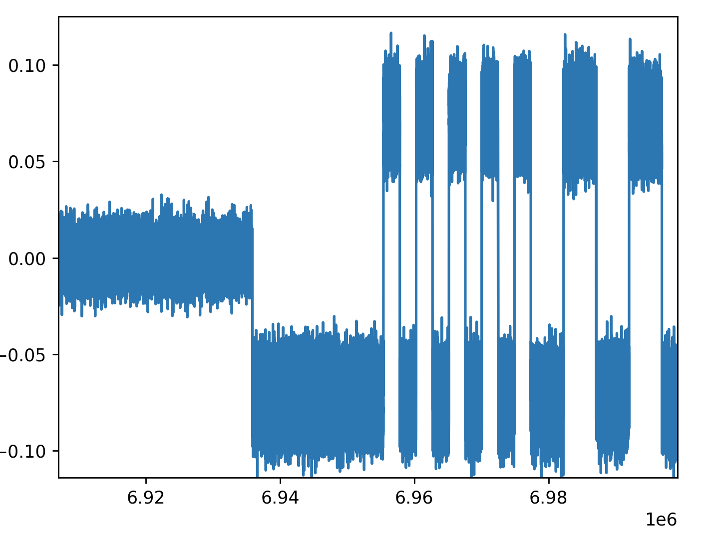
Average Idle / Carrier Detect

Our starting point for this section is the same capture as above, but post-PLL (xz compressed interleaved float32, 163,840 samples per second)

When we start out, we have IQ samples that have been mostly driven to an imaginary component of 0 and real value range between +1 and -1 for each symbol period. Our goal now is to determine if we’re receiving a signal, and if so, determine if it’s +1 or -1. This is a deceptively hard problem given it spans a lot of other similarly entertaining hard problems. I’ve opted to not solve the hard problems involved and hope that in practice my very haphazard implementation works well enough. This turns out to be both good (not solving a problem is a great way to not spend time on it) and bad (turns out it does materially impact performance). This segment is the one I plan on revisiting, first. Expect more here at some point!

Given that I want to be able to encapsulate three states in the output from this section (our Symbols are no carrier detected (“0”), real value 1 (“1”) or real value -1 ("-1")), which means spending cycles to determine what the baseline noise is to try and identify when a signal breaks through the noise becomes incredibly important.

var idleThreshold
var thresholdFactor = 10

...
    // sigThreshold is used to determine if the symbol
    // is -1, +1 or 0. It's 1.3 times the idle signal
    // threshold.
    var sigThreshold = (idleThreshold * 0.3) + idleThreshold

    // iq contains a single symbol's worth of IQ samples.
    // clock alignment isn't really considered; so we'll
    // get a bad packet if we have a symbol transition
    // in the middle of this buffer. No attempt is made
    // to correct for this yet.
    var iq []complex

    // avg is used to average a chunk of samples in the
    // symbol buffer.
    var avg float

    var mid = len(iq) / 2

    // midNum is used to determine how many symbols to
    // average at the middle of the symbol.
    var midNum = len(iq) / 50

    for j := mid; j < mid+midNum; j++ {
            avg += real(iq[j])
    }
    avg /= midNum

    var symbol float
    switch {
    case avg > sigThreshold:
        symbol = 1
    case avg < -sigThreshold:
        symbol = -1
    default:
        symbol = 0
        // update the idleThreshold using the thresholdFactor
        // to average the idleThreshold over more samples to
        // get a better idea of average noise.
        idleThreshold = (
            (idleThreshold*(thresholdFactor-1) + symbol) \
            / thresholdFactor
        )
    }

    // write symbol to output somewhere
...

Next Steps

Now that we have a stream of values that are either +1, -1 or 0, we can frame / unframe the data contained in the stream, and decode Packets contained inside, coming next in Part 4!