Writing a simulator to check phased array beamforming 🌀

While working on hz.tools, I started to move my beamforming code from 2-D (meaning, beamforming to some specific angle on the X-Y plane for waves on the X-Y plane) to 3-D. I’ll have more to say about that once I get around to publishing the code as soon as I’m sure it’s not completely wrong, but in the meantime I decided to write a simple simulator to visually check the beamformer against the textbooks. The results were pretty rad, so I figured I’d throw together a post since it’s interesting all on its own outside of beamforming as a general topic.

I figured I’d write this in Rust, since I’ve been using Rust as my primary language over at zoo, and it’s a good chance to learn the language better.

This post won’t cover the basics of how phased arrays work or the specifics of calculating the phase offsets for each antenna, but I’ll dig into how I wrote a simple “simulator” and how I wound up checking my phase offsets to generate the renders below.

Assumptions

I didn’t want to build a general purpose RF simulator, anything particularly generic, or something that would solve for any more than the things right in front of me. To do this as simply (and quickly – all this code took about a day to write, including the beamforming math) – I had to reduce the amount of work in front of me.

Given that I was concerend with visualizing what the antenna pattern would look like in 3-D given some antenna geometry, operating frequency and configured beam, I made the following assumptions:

All anetnnas are perfectly isotropic – they receive a signal that is exactly the same strength no matter what direction the signal originates from.

There’s a single point-source isotropic emitter in the far-field (I modeled this as being 1 million meters away – 1000 kilometers) of the antenna system.

There is no noise, multipath, loss or distortion in the signal as it travels through space.

Antennas will never interfere with each other.

2-D Polar Plots

The last time I wrote something like this, I generated 2-D GIFs which show a radiation pattern, not unlike the polar plots you’d see on a microphone.

These are handy because it lets you visualize what the directionality of the antenna looks like, as well as in what direction emissions are captured, and in what directions emissions are nulled out. You can see these plots on spec sheets for antennas in both 2-D and 3-D form.

Now, let’s port the 2-D approach to 3-D and see how well it works out.

Writing the 3-D simulator

As an EM wave travels through free space, the place at which you sample the wave controls that phase you observe at each time-step. This means, assuming perfectly synchronized clocks, a transmitter and receiver exactly one RF wavelength apart will observe a signal in-phase, but a transmitter and receiver a half wavelength apart will observe a signal 180 degrees out of phase.

This means that if we take the distance between our point-source and antenna element, divide it by the wavelength, we can use the fractional part of the resulting number to determine the phase observed. If we multiply that number (in the range of 0 to just under 1) by tau, we can generate a complex number by taking the cos and sin of the multiplied phase (in the range of 0 to tau), assuming the transmitter is emitting a carrier wave at a static amplitude and all clocks are in perfect sync.

    let observed_phases: Vec<Complex> = antennas
        .iter()
        .map(|antenna| {
            let distance = (antenna - tx).magnitude();
            let distance = distance - (distance as i64 as f64);
            ((distance / wavelength) * TAU)
        })
        .map(|phase| Complex(phase.cos(), phase.sin()))
        .collect();

At this point, given some synthetic transmission point and each antenna, we know what the expected complex sample would be at each antenna. At this point, we can adjust the phase of each antenna according to the beamforming phase offset configuration, and add up every sample in order to determine what the entire system would collectively produce a sample as.

    let beamformed_phases: Vec<Complex> = ...;
    let magnitude = beamformed_phases
        .iter()
        .zip(observed_phases.iter())
        .map(|(beamformed, observed)| observed * beamformed)
        .reduce(|acc, el| acc + el)
        .unwrap()
        .abs();

Armed with this information, it’s straight forward to generate some number of (Azimuth, Elevation) points to sample, generate a transmission point far away in that direction, resolve what the resulting Complex sample would be, take its magnitude, and use that to create an (x, y, z) point at (azimuth, elevation, magnitude). The color attached two that point is based on its distance from (0, 0, 0). I opted to use the Life Aquatic table for this one.

After this process is complete, I have a point cloud of ((x, y, z), (r, g, b)) points. I wrote a small program using kiss3d to render point cloud using tons of small spheres, and write out the frames to a set of PNGs, which get compiled into a GIF.

Now for the fun part, let’s take a look at some radiation patterns!

1x4 Phased Array

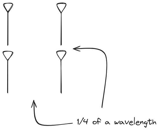
The first configuration is a phased array where all the elements are in perfect alignment on the y and z axis, and separated by some offset in the x axis. This configuration can sweep 180 degrees (not the full 360), but can’t be steared in elevation at all.

Let’s take a look at what this looks like for a well constructed 1x4 phased array:

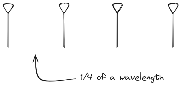
And now let’s take a look at the renders as we play with the configuration of this array and make sure things look right. Our initial quarter-wavelength spacing is very effective and has some outstanding performance characteristics. Let’s check to see that everything looks right as a first test.

Nice. Looks perfect. When pointing forward at (0, 0), we’d expect to see a torus, which we do. As we sweep between 0 and 360, astute observers will notice the pattern is mirrored along the axis of the antennas, when the beam is facing forward to 0 degrees, it’ll also receive at 180 degrees just as strong. There’s a small sidelobe that forms when it’s configured along the array, but it also becomes the most directional, and the sidelobes remain fairly small.

Long compared to the wavelength (1¼ λ)

Let’s try again, but rather than spacing each antenna ¼ of a wavelength apart, let’s see about spacing each antenna 1¼ of a wavelength apart instead.

The main lobe is a lot more narrow (not a bad thing!), but some significant sidelobes have formed (not ideal). This can cause a lot of confusion when doing things that require a lot of directional resolution unless they’re compensated for.

Going from (¼ to 5¼ λ)

The last model begs the question - what do things look like when you separate the antennas from each other but without moving the beam? Let’s simulate moving our antennas but not adjusting the configured beam or operating frequency.

Very cool. As the spacing becomes longer in relation to the operating frequency, we can see the sidelobes start to form out of the end of the antenna system.

2x2 Phased Array

The second configuration I want to try is a phased array where the elements are in perfect alignment on the z axis, and separated by a fixed offset in either the x or y axis by their neighbor, forming a square when viewed along the x/y axis.

Let’s take a look at what this looks like for a well constructed 2x2 phased array:

Let’s do the same as above and take a look at the renders as we play with the configuration of this array and see what things look like. This configuration should suppress the sidelobes and give us good performance, and even give us some amount of control in elevation while we’re at it.

Sweet. Heck yeah. The array is quite directional in the configured direction, and can even sweep a little bit in elevation, a definite improvement from the 1x4 above.

Long compared to the wavelength (1¼ λ)

Let’s do the same thing as the 1x4 and take a look at what happens when the distance between elements is long compared to the frequency of operation – say, 1¼ of a wavelength apart? What happens to the sidelobes given this spacing when the frequency of operation is much different than the physical geometry?

Mesmerising. This is my favorate render. The sidelobes are very fun to watch come in and out of existence. It looks absolutely other-worldly.

Going from (¼ to 5¼ λ)

Finally, for completeness' sake, what do things look like when you separate the antennas from each other just as we did with the 1x4? Let’s simulate moving our antennas but not adjusting the configured beam or operating frequency.

Very very cool. The sidelobes wind up turning the very blobby cardioid into an electromagnetic dog toy. I think we’ve proven to ourselves that using a phased array much outside its designed frequency of operation seems like a real bad idea.

Future Work

Now that I have a system to test things out, I’m a bit more confident that my beamforming code is close to right! I’d love to push that code over the line and blog about it, since it’s a really interesting topic on its own. Once I’m sure the code involved isn’t full of lies, I’ll put it up on the hztools org, and post about it here and on mastodon.